After the first article dedicated to the Univers project presentation, and the previous article that dealed with unsupervised learning, one will present how to reach more convincing results, using supervised learning.
“Wait. Supervised learning, without labels?”
Let’s see what we are dealing about with a quick reminder!
In the previous episod…
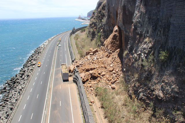
At the project origin, we got unlabelled point clouds. The aim was to automatically characterize surfaces, by distinguishing at least vegetation, cliff and scree areas.
In order to produce classification results, we detailed the point properties, by considering local neighborhoods. In the end, k-mean algorithms gave interesting insight on some datasets; however the unsupervised learning limits prevented us to be over-optimistic.
The critical question is essentially: “how to go further?”. How to produce more convincing results?
Draw hand-made labelled samples
No surprise, one must get his hands dirty!
Knowing that one handles 3D point clouds that represent natural environments, and knowing that the targetted semantic classes may be identified with a limited field expertise (as long as one does not discriminate mineral types and vegetal species…), the extraction of some labelled samples is not so expensive.
CloudCompare
CloudCompare is an Open Source software for visualizing 3D datasets. This tool is used by Géolithe engineers on a daily basis.
The following animation shows that one can extract point cloud subsamples, in a specific area. That is really important, as we know by hypothesis the nature of this area, e.g. a vegetation area. Hence all the points belonging to the sample will be subsequently labelled as vegetation thereafter.
Analyze the geometric features with respect to semantic class
At this stage of the analysis, one still have a set of unlabelled 3D point clouds, however one has some labelled subsamples for each of the class of interest. This becomes possible to study the associated geometric features (as defined in the previous article) regarding the surface label.
The next figure presents two geometric features for a set of neighborhood sizes, and for three distinct classes, extracted through CloudCompare:
- The 3D density, that corresponds to the number of points that lies into a 1m³-area around the reference point. Of course, the density is bigger when considering larger neighborhood (small neighborhoods mean small spheres of interest, and then less points). However the difference due to semantic classes is instructive: the 3D point density looks far smaller for vegetation area.
- The verticality coefficient, computed as the opposite of the normal vector third component (directly provided by the principal component analysis); its definition domain is the
[0, 1]interval. With such a feature, one sees three distinct behaviors: (i) the coefficient is high for cliff whatever the neighborhood size is, (ii) it decreases fastly when the neighborhood size grows for vegetation, (iii) it is small and roughly constant for screes.
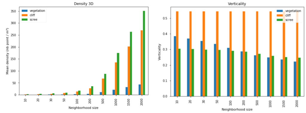
3D density and verticality coefficient, for different neighborhood size and semantic class (“pombourg” point cloud)
This approach may be generalized to each geometric feature, and to additional semantic classes. That paves the way for the usage of a supervised learning algorithm…
Train a logistic regression model
This section does not aim at comparing every possible algorithms. This is merely a proof-of-concept; the analysis output is particularly interesting if compared with unsupervised learning output (see previous article). The used algorithm here is the most symbolic classification algorithm, namely the logistic regression.
How correlated are the features?
As a first insight on how relevant is our feature set before applying logistic regressions, a correlation matrix is helpful for understanding the mathematical links underneath the features:
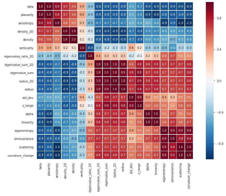
Feature correlation matrix (Pombourg scene, 1000 neighbors)
As denoted by the previous figure, one has nineteen features (that is only for one neighborhood size), amongst which highly correlated ones. Our prediction algorithm may be impacted, hence reduce the information redundancy is a concern. As an example there, considering only alpha, anisotropy, verticality and radius could be a possible simplified model.
The analysis may also be enriched by considering multiple neighborhood sizes (and filter correlated variables as well).
Let’s predict!
Here one considers a fixed set of geometric features. The CloudCompare sampling procedure was applied on 10 point clouds, that gave 28 labelled samples, in 6 different classes. Here comes the repartition:
| Label | Number of samples | Number of points |
|---|---|---|
| Vegetation | 10 | 1281k |
| Cliff | 9 | 865k |
| Scree | 4 | 143k |
| Road | 2 | 36k |
| Concrete | 2 | 155k |
| Ground | 1 | 71k |
Based on this point set, training and testing sets may be constituted (resp. 75% and 25% of the points), in order to validate the classification results. One gets 97.2% accuracy without really going into feature tuning details (full feature set, neighborhood of 20, 200, 1000 and 2000 points), the corresponding confusion matrix illustrating this score:
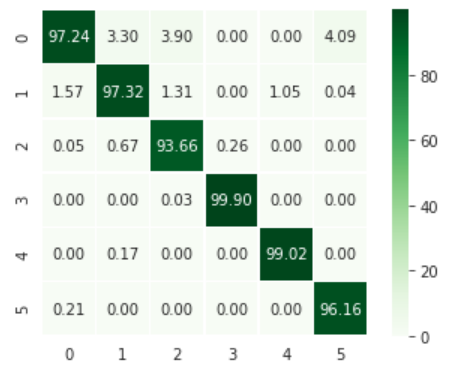
Confusion matrix associated to the prediction model (0: vegetation, 1: cliff, 2: scree, 3: road, 4: concrete, 5: ground), values expressed in %
One may also visually verify the classification results on some 3D scenes:
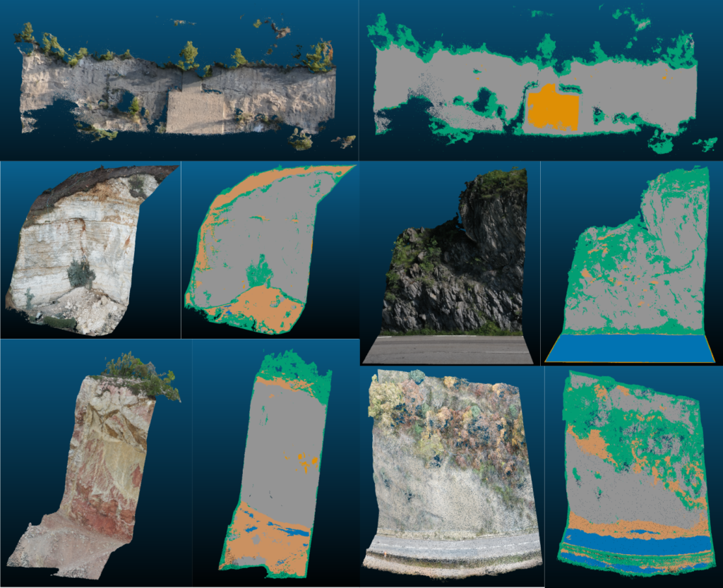
Some classification outputs (green: vegetation, grey: cliff, marron: scree, blue: road, orange: concrete)
Even if there are still some little wrong areas, the overall results look nice! They are even some ways of improving the results: thinking about the feature set, producing more labelled samples, and consequently improving the data representativeness, post-processing the outputs in order to smoothen the
borders between areas, …
Towards weak supervision
In order to close the 3D point cloud semantic segmentation chapter, a last method caught our attention, namely the weak supervision, or “how to run a deep learning method without any label (but with a strong field expertise)“.
This method was introduced by Stanford researchers, and resulted in some scientific publications as well as an Open Source framework called Snorkel. The figure below shows the overall weak supervision process, from field expertise (definition of “labelling functions”) to a model that predicts semantic classes.
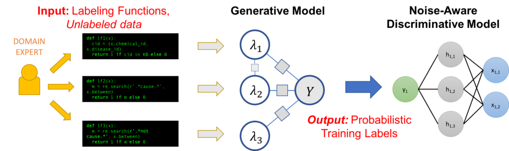
Weak supervision scheme, according to Snorkel
At this time, this is still an on-going work for us. However we got some encouraging results, thanks to the help of Géolithe engineers who provided us the expertise required for defining the labelling functions.
This method is very promising in such context, in any case this is a fascinating research topic for next months!
Conclusion
To conclude this blog post series dedicated to the Univers challenge, and our collaboration with Géolithe, we can notice that even without any labelled data, one can design prototypal supervised learning algorithms.
We tried here to be as concise as possible, however some other interesting points (e.g. performance regarding computing time, or accuracy), have not been mentionned in the articles.
If you want some additional details, feel free to leave a comment below, to consult the recently released code on Github and to contribute! And if we may be interested by a collaboration around these aspects, infos@oslandia.com is there for you!

