After a first article dedicated to Univers project presentation, let’s dig into more technical stuffs, that will mixes 3D data and hard maths towards our first machine learning algorithm.
TL;DR
The data we initially get is provided as XYZ(RGB) tables, without labelling. This makes supervised learning impossible, and forces us to analyse the underlying geometrical properties of the data. At this point, the job will be done in two steps:
- index the point cloud by the way of a tree method (e.g. kd-tree), in order to deduce local neighborhoods around each point;
- run a Principle Component Analysis (PCA) for each local neighborhoods in order to characterize each point.
After the PCA computation, one gets a set of geometric features for each point. A standard clustering algorithm (like k-means) may be run in order to associate the points to a specific class, without any prior knowledge on the data semantics.
La donnée 3D
At the beginning of the project, Géolithe provided us a bunch of 3D scenes under the .las format. This is a 3D data storage standard that considers location features (x, y and z coordinates), and extra features (typically, colors or semantic labels) as well as some metadata.
In our case, the .las files contained XYZ features for the location, RGB features for the color, and that’s pretty all. The figure below shows the kind of dataset that we are talking about. Basically, one had to recognized surfaces like vegetation, cliff, screes, road or infrastructures.
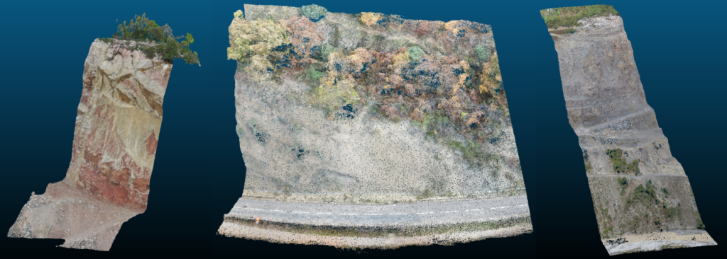
Typical 3D scenes used during the project
Reading the data is far simple in Python through the laspy package. However the visualization is more complex and needs other specific tools (e.g CloudCompare), as such datasets contains large amount of points (from 600k to more than 30M in this project context).
Catching the underlying geometrical properties
Our initial objective was to implement a Deep Learning algorithm in order to do semantic segmentation (a classification problem, plenty of data, that sounded reasonable, didn’t it?). However the unlabelled nature of the 3D point clouds made us more realistic: we could not have any training set, hence we could not “train” any predictive model.
Here comes the steps we follow in order to enrich the database.
Index the point cloud
First of all we need to index the point cloud with the help of a partitioning method in order to easily build neighborhoods around all our points. We chose the KD-tree method, and its Python implementation by the scipy library. Getting a local neighborhood can be done as follows:
from scipy.spatial import KDTree
point_cloud = ...  # Import the 3D dataset (as numpy.array)
# Build the tree
tree = scipy.spatial.KDTree(point_cloud, leaf_size=1000)
point = point_cloud[0]  # Pick a random reference point within the point cloud
# Recover the k closest points of out reference point
dist_to_neighbors, neighbor_indices = tree.query(point, k)
neighborhoods = point_cloud[neighbor_indices]
Run (a lot of) PCA
For each point, we got the local neighborhood starting from the KD-tree index. One may go deeper into the analysis by questioning the internal geometrical structure of the neighborhood.
By running a Principle Component Analysis on each local neighborhood, one can know if a given area of our point cloud is 1D-, 2D- or 3D-shaped : does it look like a tree, a wall, or is it noisy in the 3D space? Considering natural environments, one can hypothesize that cliffs and vegetations do not have the
same internal structure.
As denoted in CANUPO 1, the neighborhood size should have a great impact on the local neighborhood structure (how fine is a tree description with 20 points, 200 or 2000 points?), hence a good idea could be to consider a panel of several sizes.
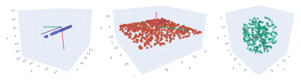
Eigenvectors after running PCA on basic 1D, 2D and 3D point clouds
In terms of Python code, the scikit-learn library does the job. However, we plan to run a huge number of PCAs (n*p where n is the number of points and p the number of neighborhood size), hence sheding light on the running time. That could be a blog post topic in itself, parallelization made a true difference in our case using the multiprocessing package.
Geometric features
After running a PCA on a local neighborhood, a large set of geometric features can be deduced. This article does not necessarily aim at listing all of them, however a small taxonomy can be drawn, mainly following 2:
- 3D geometric features deduced from the 3-dimensional PCA: barycentric coordinates (according to 1), curvature change, linearity, planarity, anisotropy, and so…;
- 2D geometric features deduced from a 2-dimensional PCA (object can also be described with respect to a plane);
- 3D/2D properties, that do not even need running any PCA: point density into neighborhoods, variability with respect to z, …;
- as an alternative neighborhood definition, that does not use KD-tree indexing and PCAs, one can also grid the point cloud, and compute the properties on bin neighborhoods…
The set of geometric feature values constitutes the point footprint.
Classify 3D points regarding their properties
At this stage, one gets a set of N points, described by M features. One may group points relatively to their feature values, by considering that the groups correspond to semantic labels (the underlying hypothesis is that these labels rely on the surface).
This description corresponds to a typical clustering algorithm. We used scikit-learn to implement it in Python, and gets the following results on previously introduced datasets, with only a few feature normalization and tuning:
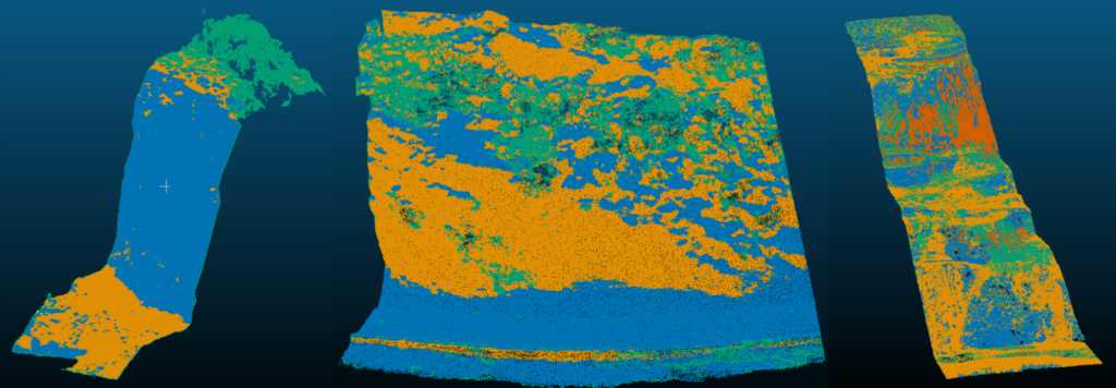
Clustered scenes starting from 3D point geometric features
If we compare these results with the raw scenes above, we see that the conclusions are highly sensitive to the scenes themselves:
- The cliff on the left (600k points, 3 clusters, 40*60*50 meters) is fairly well modelled through the k-mean: there is vegetation at the top, rock on the
middle, and screes at the bottom of the scene. - The second example (1.2M of points, 3 clusters, 40*50*30 meters) shows a cliff with a road at the bottom, and a large rocky area with some vegetation in the rest of the picture. The clustering highlight the big picture, however it is unable to finely model the scene.
- In the last example, the scene is bigger (9.8M of points, 4 clusters, 610*690*360 meters), and the surfaces are more spread in the scene. Here the results provided by the k-mean are poor.
Conclusion
When semantic labelling is not available along with the 3D data, one can still infer a semantic information by investigating on inherent geometrical patterns within the data.
The described process produces convincing results as long as we consider simple 3D scenes, with only a few data classes. In order to manage more complex cases,
investing on labelling seems unavoidable, so as to switch towards the supervised paradigm. That will be the topic of our third and last article dedicated to this project!
Feel free to leave a comment or to contact us (infos@oslandia.com) if the described methodology question you in any way!
1 Nicolas Brodu, Dimitri Lague, 2011. [3D Terrestrial lidar data classification of complex natural scenes using a multi-scale dimensionality criterion: applications in geomorphology](https://arxiv.org/abs/1107.0550). arXiv:1107.0550.
2 Martin Weinmann, Boris Jutzi, Stefan Hinz, Clément Mallet, 2015. [Semantic point cloud interpretation based on optimal neighborhoods, relevant features and efficient classifiers](http://recherche.ign.fr/labos/matis/pdf/articles_revues/2015/isprs_wjhm_15.pdf). ISPRS Journal of Photogrammetry and Remote Sensing, vol 105, pp 286-304.