Solving equations graphically with PostGIS

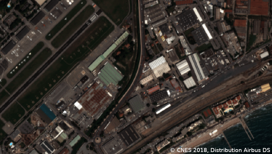
Oslandia supports the “Direction de Etudes Amont et de l’Innovation” (DEAI) of Egis Rail in the overhaul and the integration of its business tools.

For the feasibility study of the new design of public transportation lines, the objective is to have a web application allowing:

• to draw public transport lines on a base plan,
• to study the impact of the lines in terms of the population served,
• to estimate their construction and operating costs.

These needs are currently met by some desktop GIS applications, some specialized tools (for example calculation of pedestrian isochrones) and business tools developed internally.

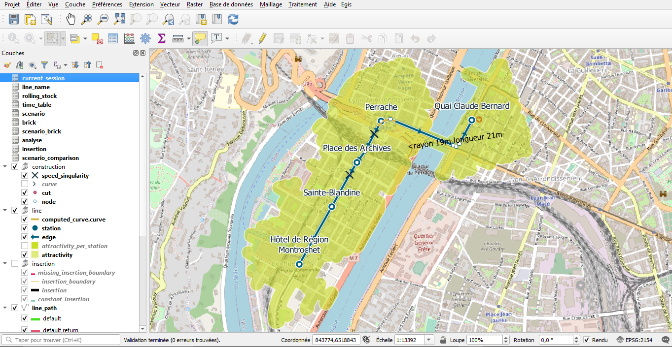
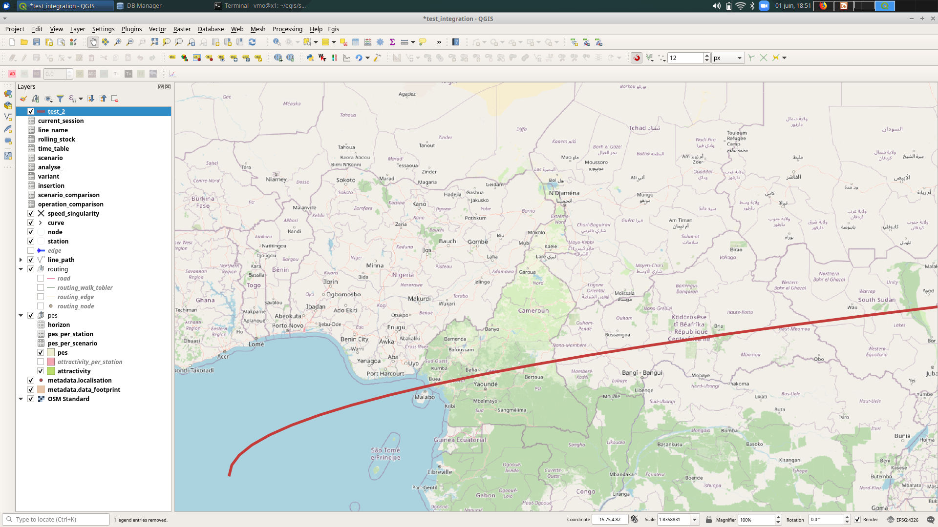
The solution being implemented is based on a PostGIS database, by fully leveraging its rich set of features to integrate processing into the data model.

This approach makes it possible to develop the model, test it and consolidate the ergonomics using QGIS as a prototype interface before developing the web application (#thickdatabase).

The context having been set, this article focuses on the calculation of travel time which is involved in estimating the operating costs of a line.

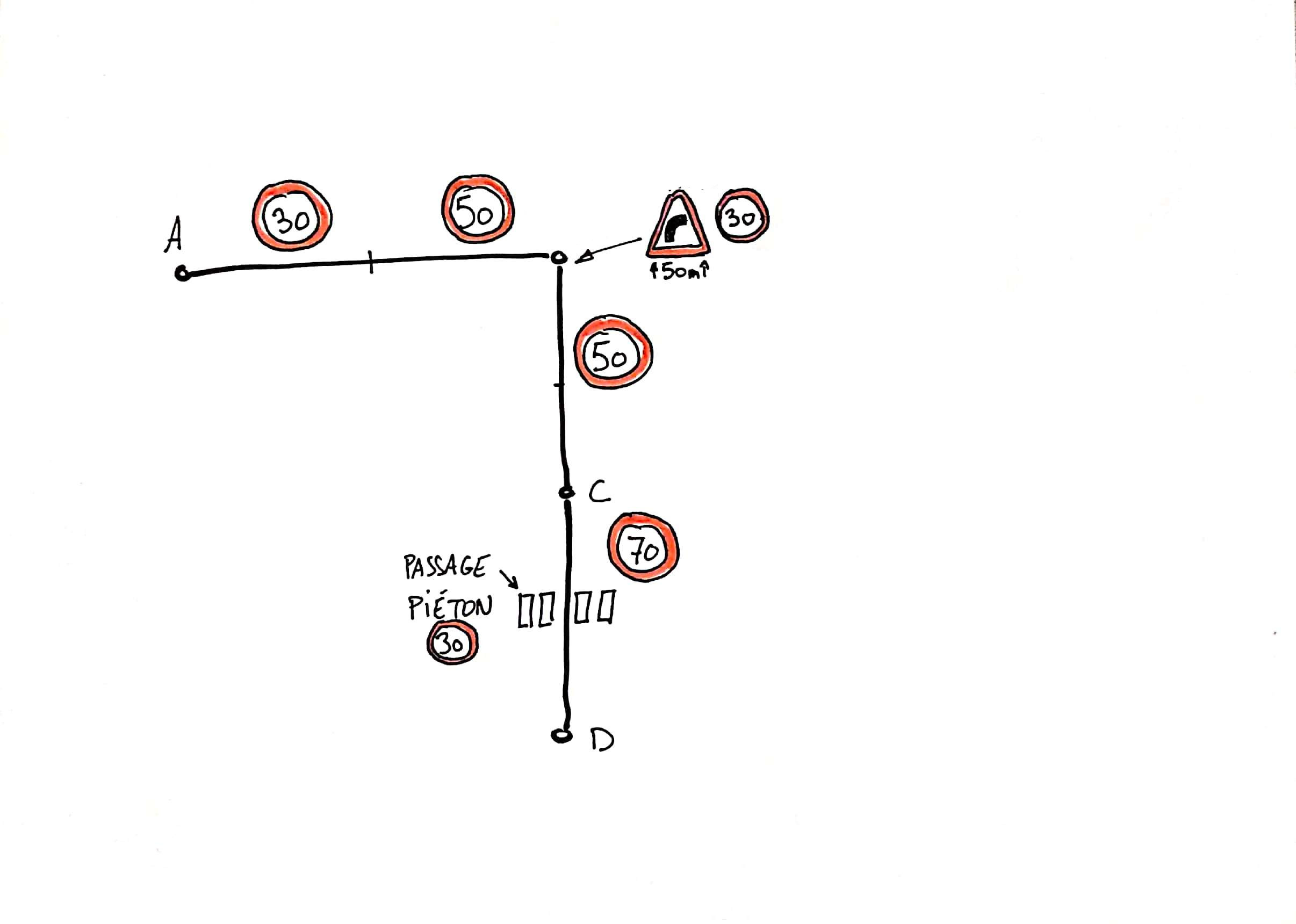
The train driver chooses between three options: speed up, slow down or maintain speed. This choice is subject to several constraints:

• station stops
• the maximum authorized speed on a section which depends on the environment (in the middle of a boulevard or in a pedestrian area)
• maximum curve speed
• maximum speed at intersections and pedestrian crossings
• stops at traffic lights (when they are red)

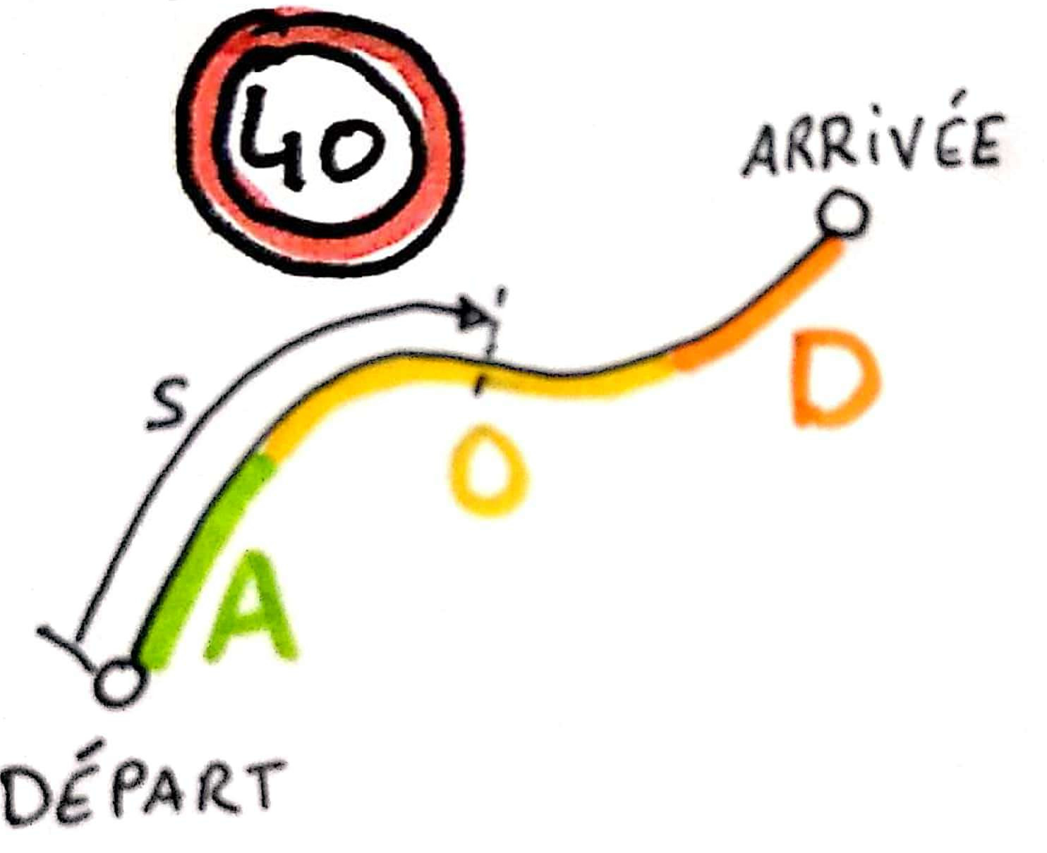
To determine the travel time, you need to know the speed at any point on the line. We’ll assume constant acceleration and deceleration. The problem that arises is therefore to determine, on the line, the areas of acceleration A, of constant speed O and of deceleration D.

Calculation of travel time in the simple case

Between two stations with a maximum speed constraint, the driver accelerates then maintains his speed when the maximum speed is reached and finally decelerates to stop.

In the simple case where the length of the section is sufficient to reach the maximum authorized speed V, the time t_A to wait for the maximum authorized speed is V/A, the length s_A traversed during t_A is:

s_A = At_A²/2

or :

s_A = V²/2A

likewise the deceleration distance s_D = V²/2D and the length traveled at constant speed s_O = s_total – s_A – s_D.

In the case where the section is not long enough to reach the maximum authorized speed, the maximum reached speed v is such that v = At_A = Dt_D where t _A and t_D are the acceleration and deceleration times respectively. To determine t_A and t_D the second equation is the total length of the section s_total = At_A²/2 + Dt_D²/2… t_A = sqrt(2Ds_{total< /sub>/(AD+A²))…}

It is almost trivial when only these two cases are to be considered:

• we assume a section long enough to calculate s_A and s_D,
• we check that s_O is positive or zero,
• if this is not the case, we use the formulas for short sections.

But there is also the case where the maximum speed is not constant between two stations, the case where it is necessary to slow down when approaching a pedestrian crossing… In short, many special cases and associated conditional structures.

It can be coded, but it lacks a bit of elegance.

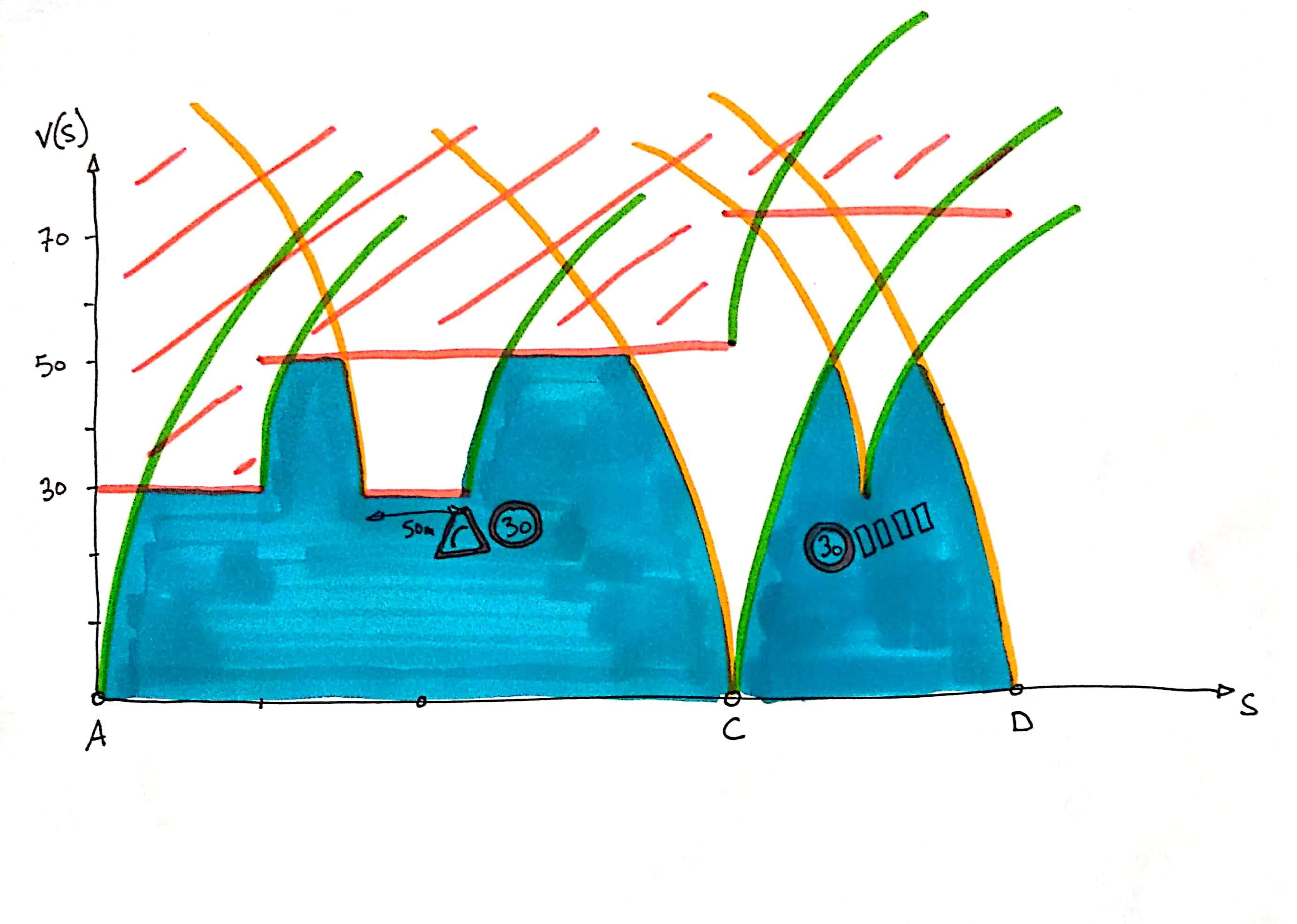
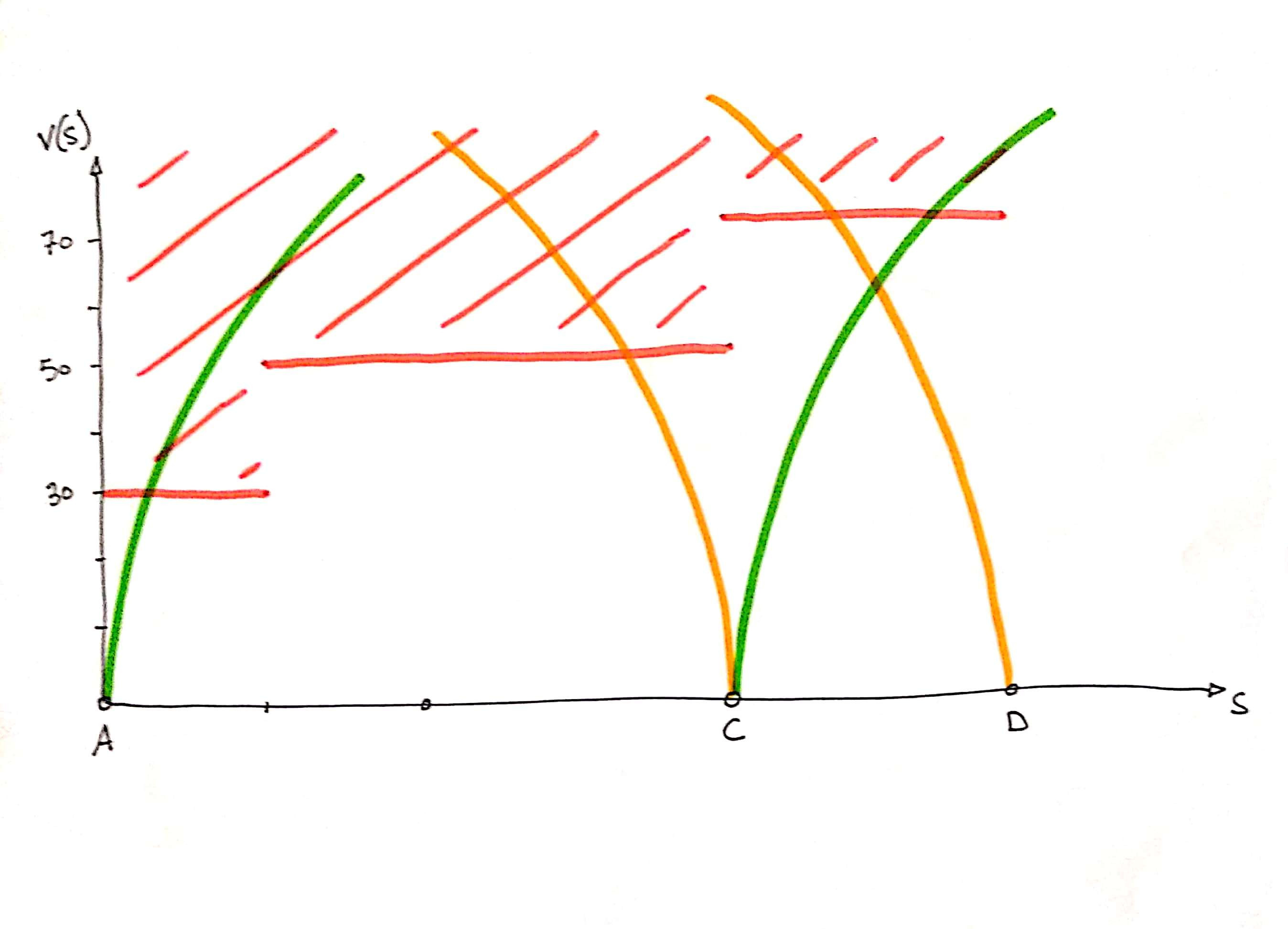
Calculation of travel time from the distance-speed curve

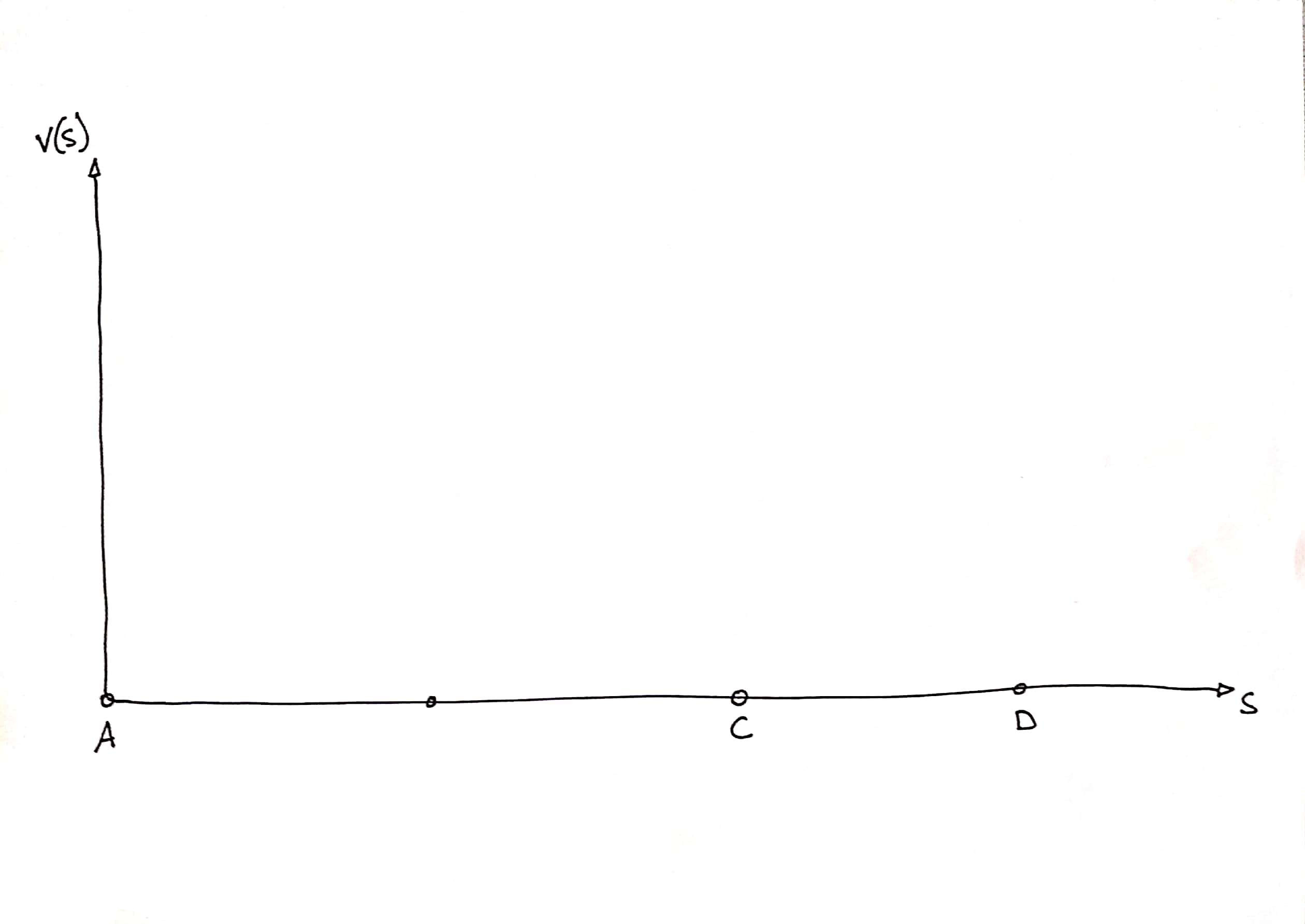
The distance-speed diagram gives the speed of the train at any point on the line.

In this diagram we can position the stations: we know their abscissas (the distances of the stations from the origin of the line) and their ordinates (zero speed).

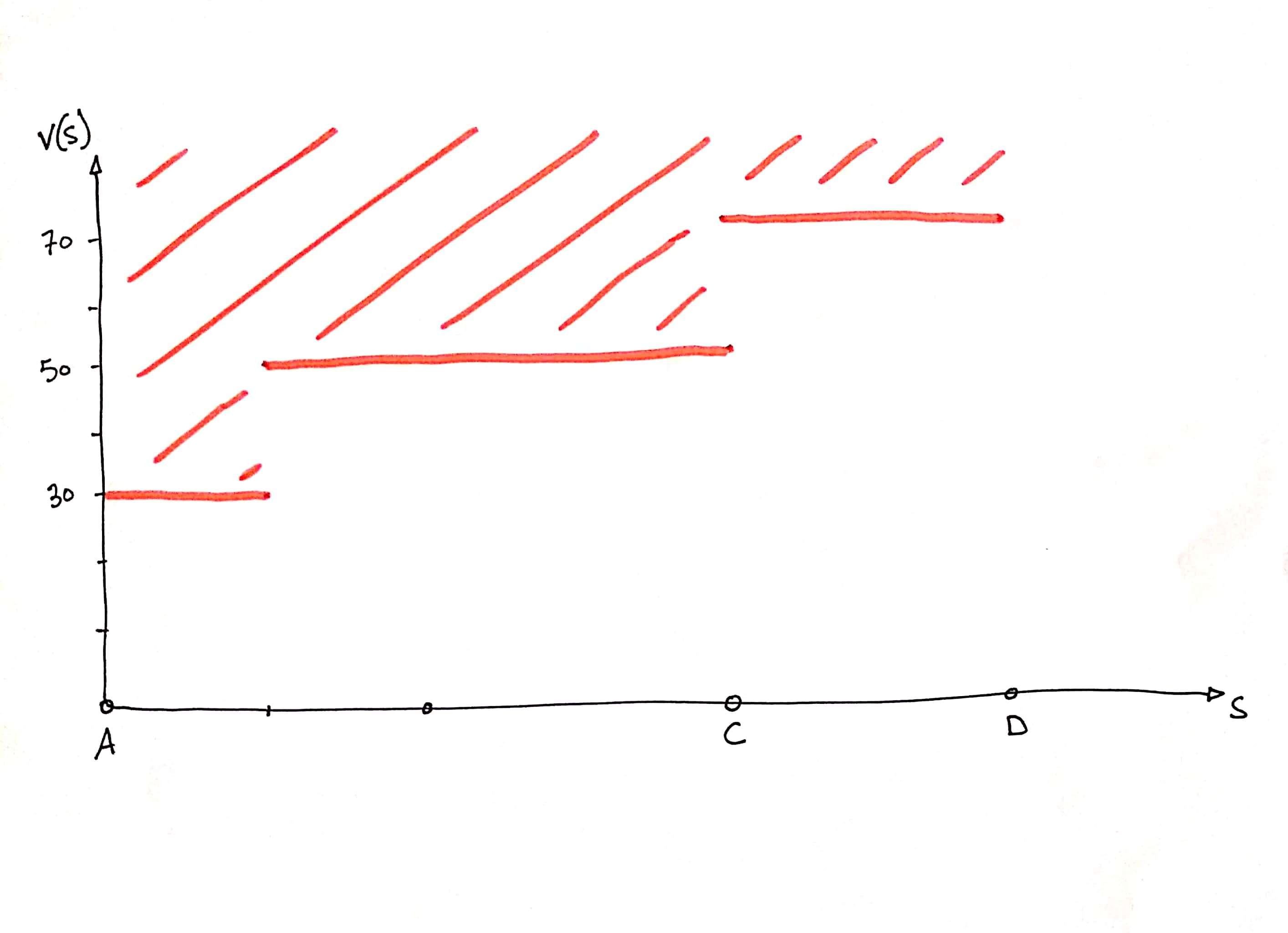
It is also possible to draw an area in which the speed curve does not pass because of the speed limits on the sections.

The velocity is a function of time, when accelerating constantly: v(t) = At + v(0) and s(t) = At²/2 + v(0)t + s(0 ).

We know how to draw this curve with PostGIS:

select st_makeline( st_makepoint( 0.5 * A *t^2, A*t ) ) from generate_series(0, 100, 0.5) t;

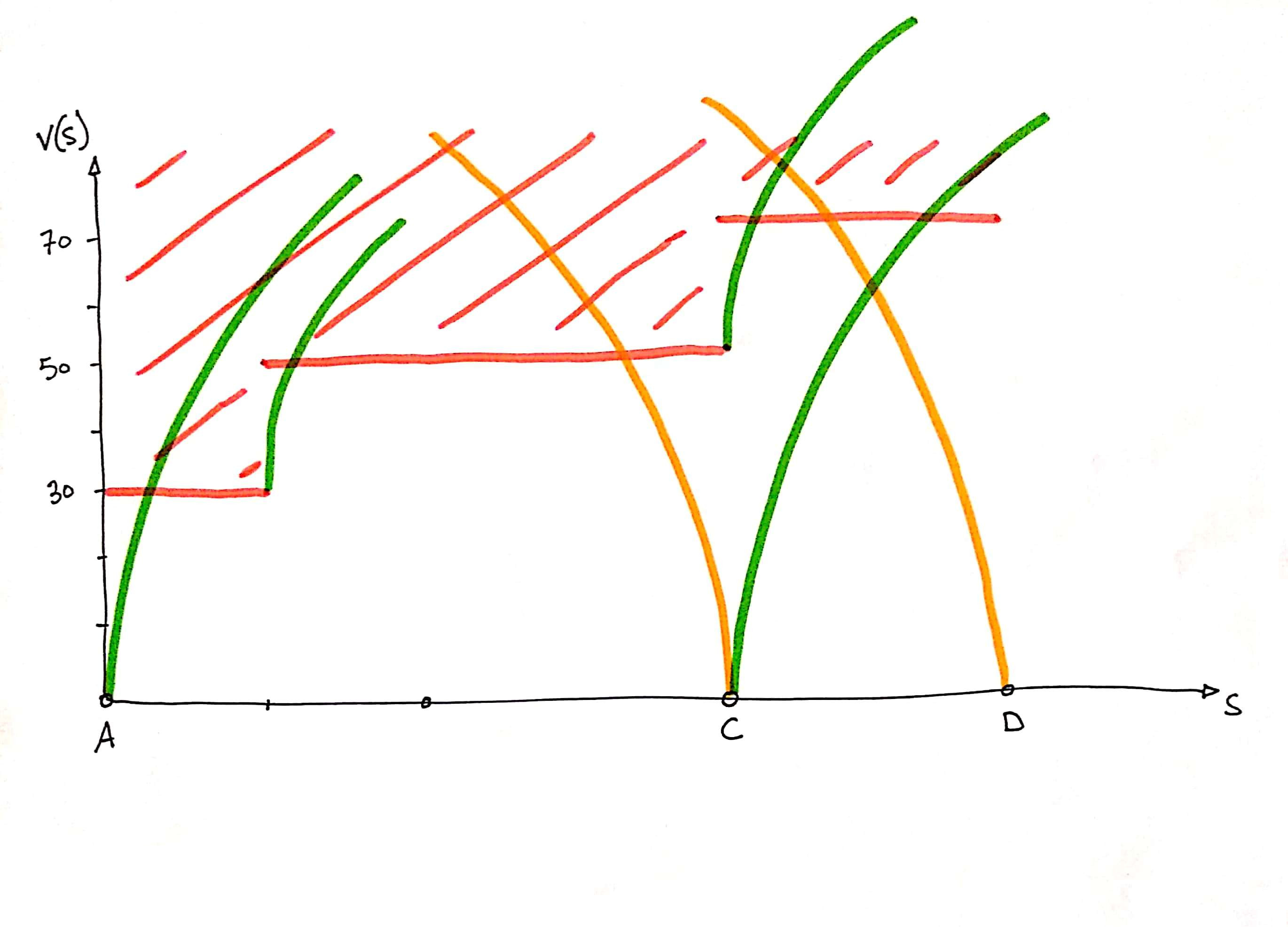
With that it is enough to trace the accelerations and decelerations from the stations:

Accelerations and decelerations linked to authorized speed limit changes:

You can easily add points (e.g. pedestrian crossing) to segments (e.g. curve), where the speed is limited with the associated acceleration and deceleration:

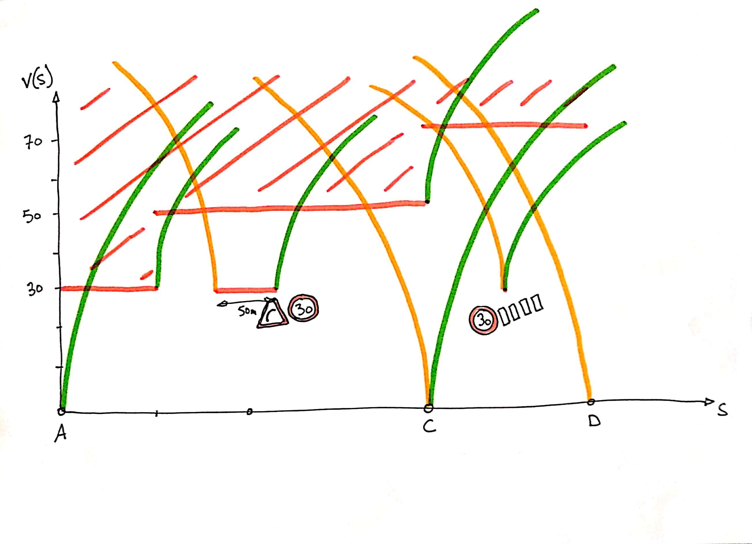
To extract the velocity curve from this set of limits, we divide the curves by each other, with st_split in order to obtain topologically clean borders, we use st_polygonize to extract the polygons defined by these borders. We only keep the polygons that are glued to the abscissa axis, in other words those for which st_length( st_intersection( polygon, axe_x ) ) > 0. The distance-velocity curve is the set of contours of these polygons from which we subtract the abscissa axis:

st_limemerge( st_difference( st_exterior_ring( polygon, x_axis ) ) )

Once the distance-speed curve has been obtained, a numerical integration is carried out to determine the travel times.

I hope that, like me, you found this diversion of PostGIS interesting which, beyond the storage and processing of geographic information, is an excellent tool for doing geometry.

If you are interested in these topics, do not hesitate to contact us (infos@oslandia.com)