At Oslandia, we like working with Open Source tool projects and handling Open (geospatial) Data. In this article series, we will play with the OpenStreetMap (OSM) map and subsequent data. Here comes the sixth article of this series, dedicated to user metadata normalization.
1 Let’s remind the user metadata
After the previous blog post, we got a set of features aiming to describe how OSM users contribute to the mapping effort. That will be our raw materials towards the clustering process. If we saved the user metadata in a dedicated .csv file, it can be recovered easily:
import pandas as pd
user_md = pd.read_csv("../src/data/output-extracts/bordeaux-metropole/bordeaux-metropole-user-md-extra.csv", index_col=0)
user_md.query('uid == 24664').T
uid                                   24664
lifespan                        2449.000000
n_inscription_days              3318.000000
n_activity_days                   35.000000
n_chgset                          69.000000
dmean_chgset                       0.000000
nmean_modif_byelem                 1.587121
n_total_modif                   1676.000000
n_total_modif_node              1173.000000
n_total_modif_way                397.000000
n_total_modif_relation           106.000000
n_node_modif                    1173.000000
n_node_modif_cr                  597.000000
n_node_modif_imp                 360.000000
n_node_modif_del                 216.000000
n_node_modif_utd                 294.000000
n_node_modif_cor                 544.000000
n_node_modif_autocor             335.000000
n_way_modif                      397.000000
n_way_modif_cr                    96.000000
n_way_modif_imp                  258.000000
n_way_modif_del                   43.000000
n_way_modif_utd                   65.000000
n_way_modif_cor                  152.000000
n_way_modif_autocor              180.000000
n_relation_modif                 106.000000
n_relation_modif_cr                8.000000
n_relation_modif_imp              98.000000
n_relation_modif_del               0.000000
n_relation_modif_utd               2.000000
n_relation_modif_cor              15.000000
n_relation_modif_autocor          89.000000
n_total_chgset                   153.000000
p_local_chgset                     0.450980
n_total_chgset_id                 55.000000
n_total_chgset_josm                0.000000
n_total_chgset_maps.me_android     0.000000
n_total_chgset_maps.me_ios         0.000000
n_total_chgset_other               1.000000
n_total_chgset_potlatch           57.000000
n_total_chgset_unknown            40.000000
Hum… It seems that some unknown features have been added in this table, isn’t it?
Well yes! We had some more variables to make the analysis finer. We propose you to focus on the total number of changesets that each user has opened, and the corresponding ratio between changeset amount around Bordeaux and this quantity. Then we studied the editors each user have used: JOSM? iD? Potlatch? Maps.me? Another one? Maybe this will give a useful extra-information to design user groups.
As a total, we have 40 features that describe user behavior, and 2073 users.
2 Feature normalization
2.1 It’s normal not to be Gaussian!
We plan to reduce the number of variables, to keep the analysis readable and interpretable; and run a k-means clustering to group similar users together.
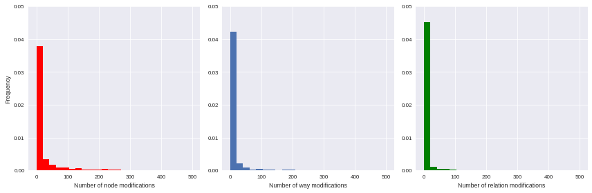
Unfortunately we can’t proceed directly to such machine learning procedures: they work better with unskewed features (e.g. gaussian-distributed ones) as input. As illustrated by the following histograms, focused on some available features, the variables we have gathered are highly left-skewed (they seems exponentially-distributed, by the way); that leading us to consider an alternative normalization scheme.
import matplotlib.pyplot as plt
import seaborn as sns
import numpy as np

%matplotlib inline
f, ax = plt.subplots(1,3, figsize=(12,4))
ax[0].hist(user_md.n_node_modif, bins=np.linspace(0,500, 25), color='r', normed=True)
ax[0].set_xlabel('Number of node modifications')
ax[0].set_ylabel('Frequency')
ax[0].set_ylim(0,0.05)
ax[1].hist(user_md.n_way_modif, bins=np.linspace(0,500, 25), normed=True)
ax[1].set_xlabel('Number of way modifications')
ax[1].set_ylim(0,0.05)
ax[2].hist(user_md.n_relation_modif, bins=np.linspace(0,500, 25), color='g', normed=True)
ax[2].set_xlabel('Number of relation modifications')
ax[2].set_ylim(0,0.05)
plt.tight_layout()
sns.set_context("paper")
2.2 Feature engineering
The basic idea we want you to keep in mind is the following one: if we find some mathematical tricks to express our variables between simple bounds (e.g. 0 and 100, or -1 and 1), we could design a smarter representation of user characteristics.
First of all you should notice that a lot of variables can be expressed as percentages of other variables:
- the number of node/way/relation modifications amongst all modifications;
- the number of created/improved/deleted elements amongst all modifications, for each element type;
- the number of changesets opened with a given editor, amongst all changesets.
def normalize_features(metadata, total_column):
    transformed_columns = metadata.columns[metadata.columns.to_series()
                                           .str.contains(total_column)]
    metadata[transformed_columns[1:]] = metadata[transformed_columns].apply(lambda x: (x[1:]/x[0]).fillna(0), axis=1)

normalize_features(user_md, 'n_total_modif')
normalize_features(user_md, 'n_node_modif')
normalize_features(user_md, 'n_way_modif')
normalize_features(user_md, 'n_relation_modif')
normalize_features(user_md, 'n_total_chgset')
Other features can be normalized starting from their definition: we know that lifespan and n_inscription_days can’t be larger than the OSM lifespan itself (we consider the OSM lifespan as the difference between the first year of modification within the area and the extraction date).
timehorizon = (pd.Timestamp("2017-02-19") - pd.Timestamp("2007-01-01"))/pd.Timedelta('1d')
user_md['lifespan'] = user_md['lifespan'] / timehorizon
user_md['n_inscription_days'] = user_md['n_inscription_days'] / timehorizon
Finally we have to consider the remaining variables that can’t be normalized as percentages of other variables, or as percentages of meaningful quantities. How can we treat them?
We choose to transform these features by comparing users to any other: knowing that a user did 100 modifications is interesting, however we could also compare it with other users, e.g. by answering the question “how many users did less modifications?”. That’s typically the definition of the empirical cumulative distribution function.
import statsmodels.api as sm

def ecdf_transform(metadata, feature):
    ecdf = sm.distributions.ECDF(metadata[feature])
    metadata[feature] = ecdf(metadata[feature])
    new_feature_name = 'u_' + feature.split('_', 1)[1]
    return metadata.rename(columns={feature: new_feature_name})

user_md = ecdf_transform(user_md, 'n_activity_days')
user_md = ecdf_transform(user_md, 'n_chgset')
user_md = ecdf_transform(user_md, 'nmean_modif_byelem')
user_md = ecdf_transform(user_md, 'n_total_modif')
user_md = ecdf_transform(user_md, 'n_node_modif')
user_md = ecdf_transform(user_md, 'n_way_modif')
user_md = ecdf_transform(user_md, 'n_relation_modif')
user_md = ecdf_transform(user_md, 'n_total_chgset')
Consequently we can characterize a user with such new dashboard:
user_md.query("uid == 24664").T
uid                                24664
lifespan                        0.661534
n_inscription_days              0.896272
u_activity_days                 0.971539
u_chgset                        0.969609
dmean_chgset                    0.000000
u_modif_byelem                  0.838881
u_total_modif                   0.966715
n_total_modif_node              0.699881
n_total_modif_way               0.236874
n_total_modif_relation          0.063246
u_node_modif                    0.967680
n_node_modif_cr                 0.508951
n_node_modif_imp                0.306905
n_node_modif_del                0.184143
n_node_modif_utd                0.250639
n_node_modif_cor                0.463768
n_node_modif_autocor            0.285592
u_way_modif                     0.971539
n_way_modif_cr                  0.241814
n_way_modif_imp                 0.649874
n_way_modif_del                 0.108312
n_way_modif_utd                 0.163728
n_way_modif_cor                 0.382872
n_way_modif_autocor             0.453401
u_relation_modif                0.984563
n_relation_modif_cr             0.075472
n_relation_modif_imp            0.924528
n_relation_modif_del            0.000000
n_relation_modif_utd            0.018868
n_relation_modif_cor            0.141509
n_relation_modif_autocor        0.839623
u_total_chgset                  0.485769
p_local_chgset                  0.450980
n_total_chgset_id               0.359477
n_total_chgset_josm             0.000000
n_total_chgset_maps.me_android  0.000000
n_total_chgset_maps.me_ios      0.000000
n_total_chgset_other            0.006536
n_total_chgset_potlatch         0.372549
n_total_chgset_unknown          0.261438
We then know that the user with ID 24664 did more node, way and relation modifications than respectively 96.7, 97.2 and 98.5% of other users, or that amongst his node modifications, 50.9% were creations, and so on…
In order to complete the normalization procedure, we add a final step that consists in scaling the features, to ensure that all of them have the same min and max values. As the features are still skewed, we do it according to a simple Min-Max rule, so as to avoid too much distorsion of our data:
from sklearn.preprocessing import RobustScaler

scaler = RobustScaler(quantile_range=(0.0, 100.0)) # = Min-max scaler
X = scaler.fit_transform(user_md.values)
3 Conclusion
This post shows you the work involved in machine learning procedure preparation. It seems quite short, however it represents a long long and unavoidable process with several try-and-error iteration loops to let the data do the talking (even an exciting job like data scientist has its dark side…)! We will exploit these new data in some machine learning procedures in the next post, dedicated to the user classification.

