Exploiting artificial intelligence within the geospatial data context tends to be easier and easier thanks to emerging deep learning techniques. Neural networks take indeed various kinds of designs, and cope with a wide range of applications.
At Oslandia we bet that these techniques will have an added-value in our daily activity, as data is of first importance for us. This article will show you an example of how we use AI techniques along with geospatial data.
Exploit an open dataset in relation to street scenes
In this article we use a set of 25,000 images provided by Mapillary, in order to investigate on the presence of some typical street-scene objects (vehicles, roads, pedestrians…). Mapillary released this dataset recently, it is still available on its website and may be downloaded freely for a research purpose.
As inputs, Mapillary provides a bunch of street scene images of various sizes in a images repository, and the same images after filtering process in instances and labels repositories. The latter is crucial, as the filtered images are actually composed of pixels in a reduced set of colors. Actually, there is one color per object types; and 66 object types in total. Some minor operations on the filtered image pixels can give outputs as one-hot vectors (i.e. a vector of 0 and 1, 1 if the corresponding label is on the image, 0 otherwise).
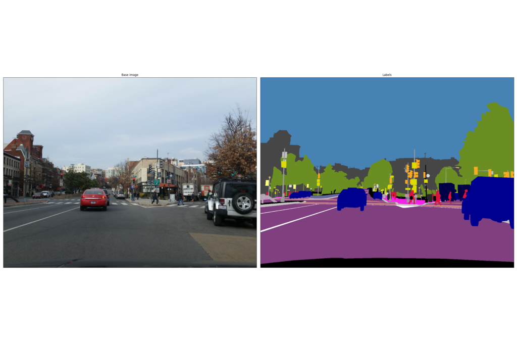
Figure 1: Example of image, with its filtered version
As a remark, neural networks consider equally-sized inputs, which is not the case of Mapillary images. A first approximation could be to resize every image as the most encountered size (2448*3264), however we choose to resize them at a smaller size (576*768) for computation purpose.
Implement a convolutional neural network with TensorFlow
Our goal here is to predict the presence of differents street-scene components on pictures. We aim to train a neural network model to make it able to detect if there is car(s), truck(s) or bicycle(s) for instance on images.
As Mapillary provided a set of 66 labels and a labelled version of each dataset image, we plan to investigate a multilabel classification problem, where the final network layer must evaluate if there is an occurrence of each label on any image.
Neural network global structure
Handling image within neural network is generally done with the help of convolutional neural networks. They are composed of several kinds of layers that must be described:
- convolutional layers, in which images are filtered by several learnable image kernels, so as to extract image patterns based on pixels (this layer type is of first importance in convolutional neural network);
- pooling layers, in order to reduce the size of images and converge towards the output layer, as well as to extract feature rough locations (the
maxpooling operation is the most common one, i.e. consider the maximal value over a local set of pixels); - fully-connected layers, where every neuron of the current layer are connected to every neuron of the previous layer.
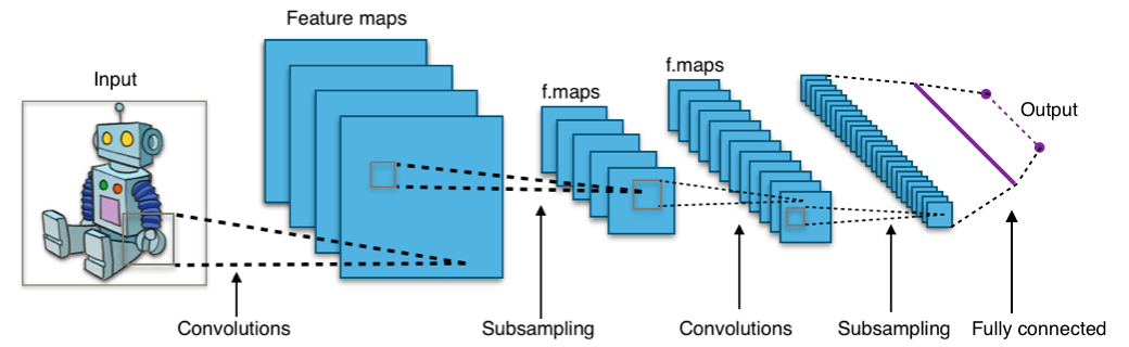
Figure 2: Convolutional neural network illustration (cf Wikipedia)
We’ve carried out a set of tests with different hyperparameter values, i.e. different amounts of each layer kinds. The results are globally stable if we consider more than one convolutional layer. Here comes the way to define a neural network with TensorFlow, the dedicated Python library.
How to define data
Inputs and outputs are defined as « placeholders », aka a sort of variables that must be fed by real data.
X = tf.placeholder(tf.float32, [None, 576, 768, 3], name='X')
Y = tf.placeholder(tf.float32, [None, 66], name='Y')
How to define a convolutional layer
After designing the kernel and the biases, we can use the TensorFlow function conv2d to build this layer.
kernel1 = tf.get_variable('kernel1', [8, 8, 3, 16], initializer=tf.truncated_normal_initializer())
biases1 = tf.get_variable('biases1', [16], initializer=tf.constant_initializer(0.0))
# Apply the image convolution with a ReLu activation function
conv_layer1 = tf.nn.relu(tf.add(tf.nn.conv2d(X, kernel1, strides=[1, 1, 1, 1], padding="SAME"),
                                biases1))
In this example, the kernel are 16 squares of 8*8 pixels considering 3 colors (RGB channels).
How to define a max-pooling layer
As for convolutional layer, there is a ready-to-use function in the TensorFlow API, i.e. max_pool.
pool_layer1 = tf.nn.max_pool(conv_layer1, ksize=[1, 4, 4, 1],
                             strides=[1, 4, 4, 1], padding='SAME')
This function takes the maximal pixel value for each block of 4*4 pixels, in every filtered image. The out-of-the-border pixels are set as the border pixels, if a block definition needs such additional information. The number of pixels is divided by 16 after such an operation.
How to define a fully-connected layer
This operation corresponds to a standard matrix multiplication; we just have to reshape the output of the previous layer so as to consider comparable structures. Let’s imagine we have added a second convolutional layer as well as second max-pooling layer, the full-connected layer definition is as follows:
reshaped = tf.reshape(pool_layer2, [-1, int((576/(4*4))*(768/(4*4))*24)])
# Create weights and biases
weights_fc = tf.get_variable('weights_fullconn', [int((576/(4*4))*(768/(4*4))*24), 1024],
                    initializer=tf.truncated_normal_initializer())
biases_fc = tf.get_variable('biases_fullconn', [1024],
                    initializer=tf.constant_initializer(0.0))
# Apply relu on matmul of reshaped and w + b
fc = tf.nn.relu(tf.add(tf.matmul(reshaped, weights_fc), biases_fc), name='relu')
# Apply dropout
fc_layer = tf.nn.dropout(fc, 0.75, name='relu_with_dropout')
Here we have defined the major part of our network. However the output layer is still missing…
Build predicted labels
The predicted labels are given after a sigmoid activation in the last layer: the sigmoid function allows to consider independant probabilities in multilabel context, i.e. if the presence of different object types on images is possible.
The sigmoid function gives probabilities of appearance for each object type, in a given picture. The predicted labels are built as simply as possible: a threshold of 0.5 is set to differentiate negative and positive predictions.
# Create weights and biases for the final fully-connected layer
weights_sig = tf.get_variable('weights_s', [1024, 66],
                              initializer=tf.truncated_normal_initializer())
biases_sig = tf.get_variable('biases_s', [66], initializer=tf.random_normal_initializer())
logits = tf.add(tf.matmul(fc_layer, weights_sig), biases_sig)
Y_raw_predict = tf.nn.sigmoid(logits)
Y_predict = tf.to_int32(tf.round(Y_raw_predict))
Optimize the network
Although several metrics may measure the model convergence, we choose to consider classic cross-entropy between true and predicted labels.
entropy = tf.nn.sigmoid_cross_entropy_with_logits(labels=Y, logits=logits)
loss = tf.reduce_mean(entropy, name="loss")
optimizer = tf.train.AdamOptimizer(0.01).minimize(loss)
In this snippet, we are using AdamOptimizer, however other solutions do exist (e.g. GradientDescentOptimizer).
Assess the model quality
Several way of measuring the model quality may be computed, see e.g.:
- accuracy (number of good predictions, over total number of predictions)
- precision (number of true positives over all positive predictions)
- recall (number of true positives over all real positive values)
They can be computed globally, or by label, as we are in a multilabel classification problem.
Train the model
Last but not least, we have to train the model we have defined. That’s a bit complicated because of batching operations, for a sake of clarity here we suppose that our training data is correctly batched and we loop over 100 iterations only, to keep the training short (that’s just for demo, prefer considering all your data -at least- once!).
from sklearn.metrics import accuracy_score

def unnest(l):
    return [index for sublist in l for index in sublist]

sess = tf.Session()
# Initialize the TensorFlow variables
sess.run(tf.global_variables_initializer())
# Train the model (over 900 batchs of 20 images, i.e. 18000 training images)
for index in range(900):
    X_batch, Y_batch = sess.run([train_image_batch, train_label_batch])
    sess.run(optimizer, feed_dict={X: X_batch, Y: Y_batch})
    if index % 10 == 0:
        Y_pred, loss_batch = sess.run([Y_predict, loss], feed_dict={X: X_batch, Y: Y_batch})
        accuracy_batch = accuracy_score(unnest(Y_batch), unnest(Y_pred))
        print("""Step {}: loss = {:5.3f}, accuracy={:1.3f}""".format(index, loss_batch, accuracy_batch))
What kind of objects are on a test image ?
In order to illustrate the previous developments, we can test our network on a new image, i.e. an image that does not have been scanned during model training.
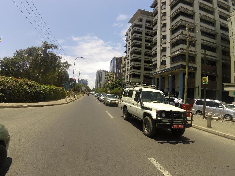
Figure 3: Example of image used to validate the model
The neural network is supplied with this image and the corresponding true labels, to compute predicted labels:
Y_pred = sess.run([Y_predict], feed_dict={X: x_test, Y: y_test})
sess.close()
The model accuracy for this image is around 74,2% ((34+15)/66), which is quite good. However it may certainly be improved as the model has seen the training images only once…
              Y_pred=False  Y_pred=True
y_test=False            34            9
y_test=True              8           15
We can extract the more interesting label category, aka the true positives corresponding to object on the image detected by the model:
0              curb
1              road
2          sidewalk
3          building
4            person
5           general
6               sky
7        vegetation
8         billboard
9      street-light
10             pole
11     utility-pole
12    traffic-light
13            truck
14        unlabeled
dtype: object
To understand the category taxonomy, interested readers may read the dedicated paper available on Mapillary website.
How to go further?
In this post we’ve just considered a feature detection problem, so as to decide if an object type t is really on an image p, or not. The natural prolongation of that is the semantic segmentation, i.e. knowing which pixel(s) of p have to be labeled as part of an object of type t.
This is the way Mapillary labelled the pictures; it is without any doubt a really promising research field for some use cases related to geospatial data!
To go deeper into this analysis, you can find our code on Github.
If you want to collaborate with us and be a R&D partner on such a topic, do not hesitate to contact us at infos@oslandia.com!

