After focusing on street-scene images, our deep learning framework is currently exploited in order to analyze aerial images and building footprints with semantic segmentation algorithms.
We recently extend these last works by investigating an instance-segmentation use case.
Context
In parallel to the last FOSS4G conference at Dar es Salaam (Tanzania), WeRobotics recently organized the Open AI Tanzania challenge.
The goal of the challenge was to automatically recognize individual instances of building footprints on some tanzanian areas by discriminating complete and unfinished buildings, as well as foundations.
Technical challenge
Two major differences arise between this context and the work done around building footprint detection with Deeposlandia:
- discrimination of building types;
- instance-specific segmentation instead of semantic segmentation.
The former point is not so tricky, as many more labels have to be handled in the street-scene dataset we used. However the latter one needs a far more sophisticated algorithm than semantic segmentation algorithms are. We choose to apply one of the best state-of-the-art solution in this way: Mask-RCNN.
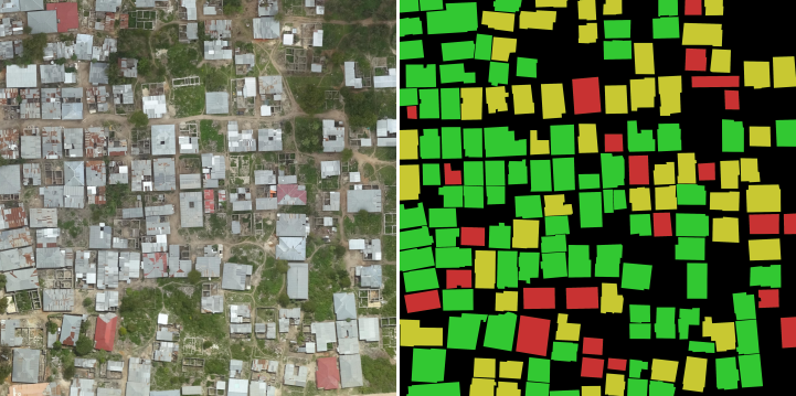
Example of image in the Tanzania dataset: (a) raw images, (b) rasterized labels
Data pipeline
Raw data is available on request on the challenge website.
The whole process has been implemented in Python as a Luigi pipeline. It is depicted in the next scheme.
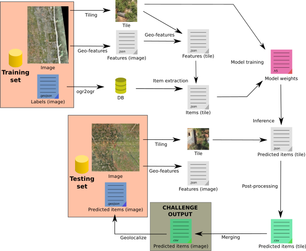
Scheme of our data pipeline
So as to recover testing image buildings with their geographical location, several steps are required.
First raw images are tiled so as to supply the deep learning model with sustainably-sized images. Geographical features (coordinates, SRID) are extracted from the raw images, in order to deduce the same information at the tile level.
Parallely labels -provided as .geojson files- are stored into a database that is thereafter queried to get each tile item.
Starting from pairs of tiles and item sets, a Mask-RCNN model is trained to recognized finished building, incomplete building and foundation instances. The model training is implemented with Python/Keras, this step output is a binary hdf5 file containing every layer weight.
Then these weights are used in order to make the neural network infer building instances on testing dataset. This produces one resulting .json file per testing tile; those files describe the label scores and the geographical location for each predicted instance.
Last but not least, these instances are aggregated for each raw testing images. Duplicated instance on adjacent tiles must be filtered here. At this point, we get a .csv file per raw testing image; this is the challenge output.
One could even go one step further by generating .geojson files so as to visually compare predicted items with rasters in QGIS, as depicted in the following figure!
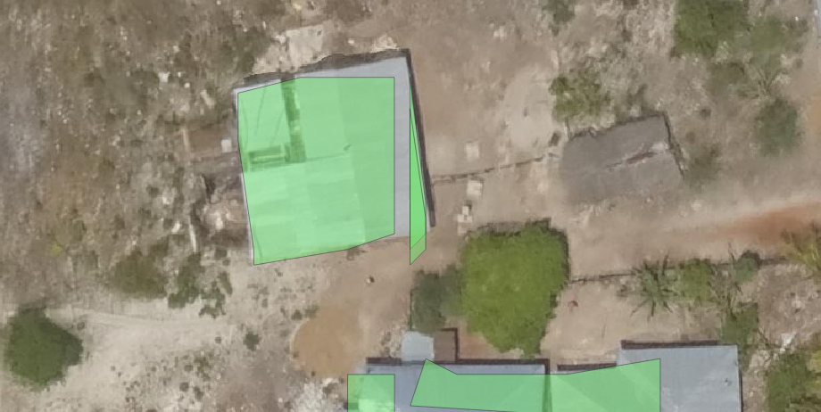
Example of two tiles with predicted building instances (without adjacent prediction filtering)
What next?
Our objective during this challenge was not necessarily to provide a ready-to-use predictor, as we began the challenge quite late. However we are proud to announce the oncoming release of the Proof-of-Concept of our data pipeline.
In the next weeks we will be focused on the development of this research code, so as to provide an industrialized version of the deep learning data pipeline.
If you have questions regarding deep learning methods or geospatial data pipeline, do not hesitate to contact us (infos+data@oslandia.com)!

