First of all we have to recover a dataset. Two major solutions exist: either we dowload a regional area on Geofabrik (e.g. a continent, a country, or even a sub-region) in osm or osh version (i.e. up-to-date API or history), or we extract another free area with the help of osmium-tool. Even if the former solution is easier to implement, the latter one permits to work with alternative data sets. We detail this method in subsequent paragraphes.

Note: osmium-tool is available as a package in the Debian GNU/Linux distribution.

Let us work with Bordeaux, a medium-sized French city. This alternative method needs the area geographical coordinates. We recover them by drawing the accurate bounding box within the OpenStreetMap API export tool. We get the following bounding box coordinates: the top-left corner is at {44.9335,-0.7179} whilst the bottom-right corner is at {44.7216, -0.4134}. These coordinates seem quite weird (weirdly concise!), however they are just hand-made, by successive zooms in the OSM API.

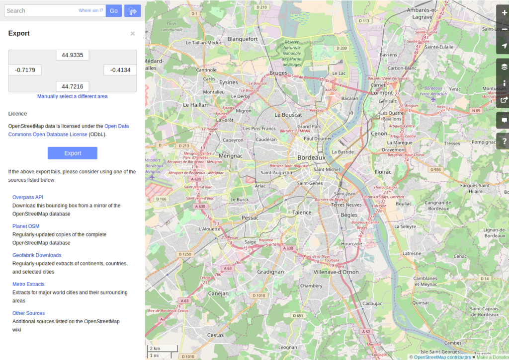
Hand-made bounding box on Bordeaux city (France)

{
  "extracts": [
    {
      "output": "bordeaux-metropole.osh.pbf",
      "output_format": "osh.pbf",
      "description": "extract OSM history for Bordeaux (France)",
      "bbox": {"left": -0.7179,
               "right": -0.4134,
               "top": 44.9335,
               "bottom": 44.7216}
     }
  ],
  "directory": "/path/to/outputdir/"
}

This JSON file is used by osmium to build a standard pbf file in the following shell command:

osmium extract --with-history --config=region.json latest-planet.osh.pbf

Where latest-planet.osh.pbf is the input file (downloaded from Geofabrik website, we still need some original data!). region.json refers to the previously defined JSON file. The --with-history flag here is important as well. We want to study the temporal evolution of some OSM entities, the number of contributions, and check some specific OSM entities such as nodes, ways or relations and get their history.

At this point, we have a pbf file that contains every OSM element versions through time. We still have to write them into a csv file. Here we use pyosmium (see previous article).

This operation can be done through a simple Python file (see snippets below).

import osmium as osm
import pandas as pd

class TimelineHandler(osm.SimpleHandler):
    def __init__(self):
        osm.SimpleHandler.__init__(self)
        self.elemtimeline = []

    def node(self, n):
        self.elemtimeline.append(["node",
                                  n.id,
                                  n.version,
                                  n.visible,
                                  pd.Timestamp(n.timestamp),
                                  n.uid,
                                  n.changeset,
                                  len(n.tags)])

First we have to import the useful libraries, that are pandas (to handle dataframes and csv files) and pyosmium. Then, we define a small OSM data handler, that saves every nodes into the elemtimeline attribute (i.e. a list). This example is limited to nodes for a sake of concision, however this class is easily extensible to other OSM objects. We can observe that several node attributes are recorded: the element type (« node » for nodes, of course!), ID, version in the history, if it is currently visible on the API, timestamp (when the version has been set), user ID, change set ID and the number of associated tags. These attributes are also available for ways and relations, letting the chance to put a little more abstraction in this class definition!

An instance of this class can be created so as to save OSM nodes within the Bordeaux metropole area (see below). We pass the input file name to the apply_file procedure, that scans the input file and fills the handler list accordingly. After that we just have to transform the list into a pandas DataFrame, to make further treatments easier.

tlhandler = TimelineHandler()
tlhandler.apply_file("../src/data/raw/bordeaux-metropole.osh.pbf")
colnames = ['type', 'id', 'version', 'visible', 'ts', 'uid', 'chgset', 'ntags']
elements = pd.DataFrame(tlhandler.elemtimeline, columns=colnames)
elements = elements.sort_values(by=['type', 'id', 'ts'])
elements.head(10)

   type        id  version  visible                        ts    uid  chgset  ntags
0  node  21457126        2    False 2008-01-17 16:40:56+00:00  24281  653744      0
1  node  21457126        3    False 2008-01-17 16:40:56+00:00  24281  653744      0
2  node  21457126        4    False 2008-01-17 16:40:56+00:00  24281  653744      0
3  node  21457126        5    False 2008-01-17 16:40:57+00:00  24281  653744      0
4  node  21457126        6    False 2008-01-17 16:40:57+00:00  24281  653744      0
5  node  21457126        7     True 2008-01-17 16:40:57+00:00  24281  653744      1
6  node  21457126        8    False 2008-01-17 16:41:28+00:00  24281  653744      0
7  node  21457126        9    False 2008-01-17 16:41:28+00:00  24281  653744      0
8  node  21457126       10    False 2008-01-17 16:41:49+00:00  24281  653744      0
9  node  21457126       11    False 2008-01-17 16:41:49+00:00  24281  653744      0

With the help of pandas library, to save the file into csv format is straightforward:

elements.to_csv("bordeaux-metropole.csv", date_format='%Y-%m-%d %H:%M:%S')

At this point, the OSM data history is available in a csv file format, coming with a whole set of attributes that will be useful to describe the data.

From the OSM data history we can recover the current state of OSM data (or more precisely, the API state at the data extraction date). The only needed step is to select the up-to-date OSM objects, i.e. those with the last existing version, through a group-by operation.

def updatedelem(data):
    updata = data.groupby(['type','id'])['version'].max().reset_index()
    return pd.merge(updata, data, on=['id','version'])
uptodate_elem = updatedelem(elements)
uptodate_elem.head()

  type_x        id  version type_y  visible                        ts    uid   chgset ntags
0   node  21457126       48   node    False 2008-01-17 16:42:01+00:00  24281   653744     0
1   node  21457144        9   node    False 2008-01-17 16:45:43+00:00  24281   653744     0
2   node  21457152        7   node    False 2008-03-06 20:51:58+00:00  25762   277530     0
3   node  21457164        5   node    False 2008-01-17 16:48:00+00:00  24281   653744     0
4   node  21457175        4   node    False 2008-01-17 16:47:51+00:00  24281   653744     0

This seem to be a quite useless function: we could have found directly such data on GeoFabrik website, isn’t it? … Well, it is not that useless. As an extension of this first procedure, we propose a simple but seminal procedure called datedelems that allows us to get the OSM API picture given a specific date:

def datedelems(history, date):
    datedelems = (history.query("ts <= @date")
                  .groupby(['type','id'])['version']
                  .max()
                  .reset_index())
    return pd.merge(datedelems, history, on=['type','id','version'])

oldelem = datedelems(elements, "2008-02-01")
oldelem.head()

   type        id  version  visible                        ts    uid  chgset  ntags
0  node  21457126       48    False 2008-01-17 16:42:01+00:00  24281  653744      0
1  node  21457144        9    False 2008-01-17 16:45:43+00:00  24281  653744      0
2  node  21457152        6     True 2008-01-17 16:45:39+00:00  24281  653744      1
3  node  21457164        5    False 2008-01-17 16:48:00+00:00  24281  653744      0
4  node  21457175        4    False 2008-01-17 16:47:51+00:00  24281  653744      0

We can notice in this function that pandas allows to express queries in a SQL-like mode, a very useful practice in order to explore data! As a corollary we can build some time series aiming to describe the evolution of the API in terms of OSM objects (nodes, ways, relations) or users.

What if we consider OSM API state month after month? What is the temporal evolution of node, way, or relation amounts? The following procedure helps us to describe the OSM API at a given date: how many node/way/relation there are, how many user have contributed, how many change sets have been opened. Further statistics may be designed, in the same manner.

def osm_stats(osm_history, timestamp):
    osmdata = datedelems(osm_history, timestamp)
    nb_nodes = len(osmdata.query('type == "node"'))
    nb_ways = len(osmdata.query('type == "way"'))
    nb_relations = len(osmdata.query('type == "relation"'))
    nb_users = osmdata.uid.nunique()
    nb_chgsets = osmdata.chgset.nunique()
    return [nb_nodes, nb_ways, nb_relations, nb_users, nb_chgsets]

osm_stats(elements, "2014-01-01")

Here we do not get any way or relation, that seems weird, doesn’t it? However, do not forget how the parser was configured above ! By tuning it so as to consider these OSM element types, this result is modified. As a corollary this configuration only counts the users and change sets that contribute to nodes !

By designing a last function, we can obtain a pandas dataframe that summarizes basic statistics at regular timestamps: in this example, we focus on monthly evaluations, however everything is possible… A finner analysis is possible, by taking advantage of pandas time series capability.

def osm_chronology(history, start_date, end_date):
    timerange = pd.date_range(start_date, end_date, freq="1M").values
    osmstats = [osm_stats(history, str(date)) for date in timerange]
    osmstats = pd.DataFrame(osmstats, index=timerange,
                            columns=['n_nodes', 'n_ways', 'n_relations',
                                     'n_users', 'n_chgsets'])
    return osmstats

These developments open further possibilities. Areas are comparable through their history. A basic hypothesis could be: some areas have been built faster than others, e.g. urban areas vs desert areas. To investigate on the evolutions of their OSM objects appears as a very appealing way to address this issue!

To illustrate the previous points, we can call the osm_chronology procedure to Bordeaux-related OSM data. We can study the last 10 years, as an example:

chrono_data = osm_chronology(elements, "2007-01-01", "2017-01-01")

pd.concat([chrono_data.iloc[:10,[0,3,4]], chrono_data.iloc[-10:,[0,3,4]]])

            n_nodes  n_users  n_chgsets
2007-01-31       24        1          2
2007-02-28       24        1          2
2007-03-31       45        3          4
2007-04-30       45        3          4
2007-05-31     1744        4          8
2007-06-30     1744        4          8
2007-07-31     1744        4          8
2007-08-31     3181        6         12
2007-09-30     3186        7         15
2007-10-31     3757        8         18
2016-03-31  2315763      882      15280
2016-04-30  2318044      900      15468
2016-05-31  2321910      918      15841
2016-06-30  2325689      931      16153
2016-07-31  2329592      942      16613
2016-08-31  2334206      955      16835
2016-09-30  2337157      973      17005
2016-10-31  2339526     1004      17462
2016-11-30  2342109     1014      17637
2016-12-31  2349670     1028      17933

The figure below describes the evolution of nodes, ways and relations around Bordeaux between 2007 and 2017, as well as the number of users and change sets. The graphes are log-scaled, for a sake of clarity.

We can see that the major part of Bordeaux cartography has been undertaken between fall of 2010 and spring of 2013, with a clear peak at the beginning of 2012. This evolution is highly pronounced for nodes or even ways, whilst the change set amount and the contributor quantity increased regularly. This may denote the differences in terms of user behaviors: some of them create only a few objects, while some others contributes with a large amount of created entities.

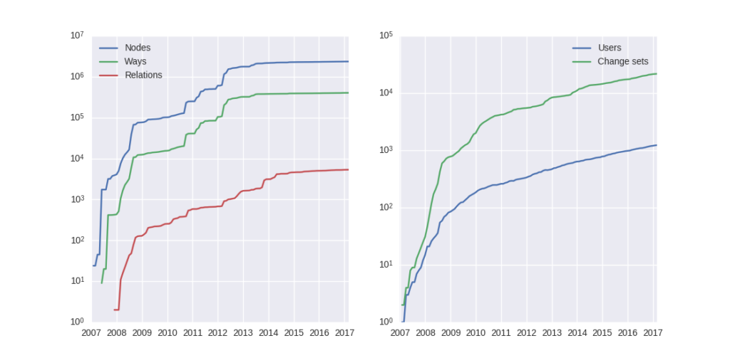
Amount of OSM objects in the area of Bordeaux (France)

As a remark, the number of active contributors plotted here is not really representative of the total of OSM contributors: we consider only local data here. Active users all around the world are not those who have collaborated for this specific region. However the change set and user statistics for full-planet dumps exist, if you are interested in going deeper about this point!

Before concluding this article, here is provided a comparison between OSM node amounts in several french areas. We just mention small areas, to keep the evaluation short: Upper Normandy, a roughly rural environment with some medium-sized cities (Rouen, Le Havre, Evreux…), Corsica, an montainous island near to mainland France and French Guiana, an overseas area mainly composed of
jungle. The figure below shows the difference between these areas in terms of OSM nodes and active contributors. To keep the comparison as faithful as possible, we have divided these amounts by each surface area: respectively 12137, 8680 and 83534 square kilometers for Upper Normandy, Corsica and French Guiana.

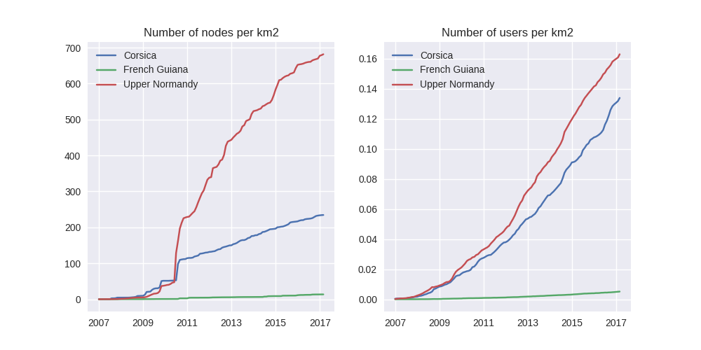
Without any surprise, it is the mainland area (Upper Normandy) that is the most dense on OSM. This area contains almost 700 nodes per square kilometer (quite modest, however we talk about a rural area!). We can notice that they are almost the same number of contributors between Normandy and Corsica. On the other hand, French Guiana is an extrem example, as expected! There are less than 15 nodes and 0.01 contributor per square kilometer. We have identified a OSM desert, welcome to the Guiana jungle ! (You can act on it: be environment-friendly, plant some more trees!)